How ensemble sensitivity analysis works

An ensemble forecast is 50 slightly different versions of the future. ESA uses that spread to ask which earlier features of the forecast decide how a particular local outcome turns out: the depth of a low over the UK, the peak of a heatwave, or where a typhoon goes.

50ECMWF ensemble members (open data)

T+0–2406-hourly, latest 00Z or 12Z run

0.25°grid for the response box, to T+120, over land and coasts

1°grid for sensitivity maps, 0–90°N, to T+240

The idea in one picture

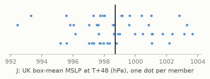
Pick a forecast quantity that matters to you and reduce it to one number per member. This is the response function J. In the demo case below, J is the mean sea-level pressure over a 5° box covering the UK at T+48 (…). The members disagree: the ensemble mean is … hPa, with a spread of … hPa.

Strip chart of J for each of the 50 members — J for each member. ESA tries to explain this spread.

Now take any earlier field at any grid point, for example 500 hPa height at … at T+24, and plot it against J for all 50 members. If members with a higher Z500 there go on to have higher pressure over the UK, the points line up. The slope of the regression line is the sensitivity.

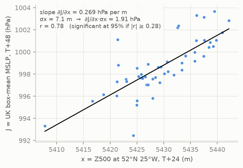
Scatter plot of J against Z500 at one point, with regression line — Each dot is one member. ESA computes this regression at every grid point, for every variable and step, and maps the result.

Sensitivity ∂J/∂x = cov(J, x) / var(x)
Standardised ∂J/∂x · σx = cov(J, x) / σx (change in J for a 1 s.d. change in x)
Correlation r = cov(J, x) / (σJ σx)

Ancell & Hakim (2007); Torn & Hakim (2008). This is a linear regression across the ensemble. It shows association within the forecast, which, through the model's dynamics, usually reflects cause and effect.

Using the tool

Explore Before you draw a box, the map shows the response variable's ensemble mean (contours) and spread (shaded) at the chosen "Valid at" time, e.g. MSLP at T+72. This lets you place the box on the feature you care about and see where the members disagree. Switch to State spread to animate the chosen state variable through every step instead.

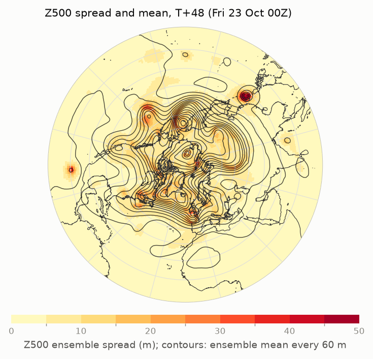
Z500 spread at T+48. Spread is concentrated in troughs and developing systems.
Define J Choose a variable, the box statistic (mean, max or min) and the time. Click Draw box and drag on the map, or type the edges. For rain, use 24 hour precipitation: the total over the 24 hours ending at the chosen time.
Pick x Choose the state variable to test, such as 500 hPa height for the upper-level pattern or MSLP for surface systems.
Animate Step back from the response time towards T+0 to trace where the signal comes from.
Read Hover over the map to read the ensemble mean, the sensitivity and r at any point.

Reading the sensitivity maps

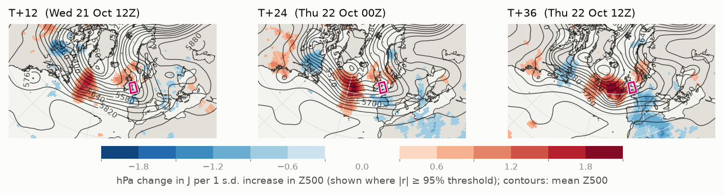
Three maps of standardised sensitivity of UK MSLP to Z500 at T+12, T+24 and T+36 — Standardised sensitivity of UK box-mean MSLP at T+48 (pink box) to Z500, shown where significant at 95%. Contours show the ensemble-mean Z500.

Red: a higher value of x here goes with a higher J. Blue: a higher value of x here goes with a lower J.

Here the red area sits in the Atlantic trough upstream of the UK. Members with higher heights there, meaning a weaker trough or one that has already moved further east, give higher pressure over the UK two days later. The blue areas downstream have the opposite sign. A red–blue pair across a trough like this usually means the outcome depends on the trough's position and speed (its phase), not just its depth. Stepping from T+12 to T+36, the pattern moves east with the trough towards the box, which is how ESA traces a signal back to its source.

The value at each point is the change in J for a typical (1 s.d.) change in x there. A value of … hPa means a one-standard-deviation increase in Z500 at that point goes with about … hPa higher pressure over the UK.

Which shading to use

Shading	Units	Use it for
Standardised sensitivity	units of J	The default. Comparable across places and variables, because it allows for how much x actually varies.
Sensitivity ∂J/∂x	J per unit of x	The physical gradient, e.g. "hPa per m of Z500". It can look large where x barely varies, which matters little in practice.
Correlation r	−1 to 1	The strength of the link, independent of units. It is what the significance test uses.

Signal or noise?

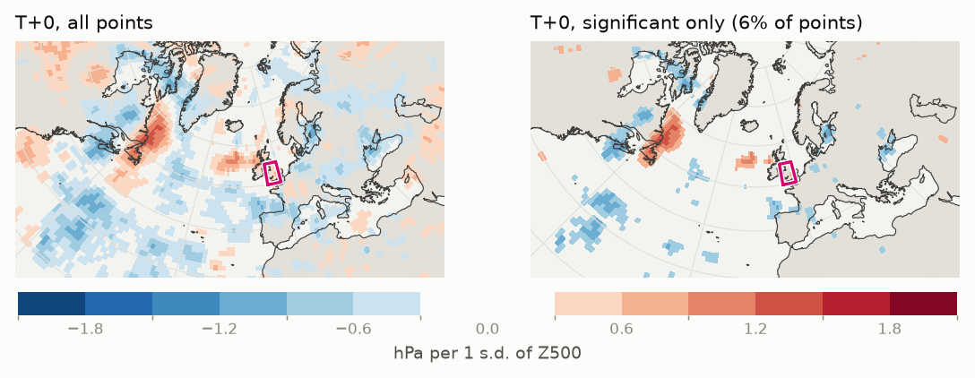
With 50 members, a correlation needs |r| ≥ … to be significant at 95%. That also means about 5% of all grid points pass by chance alone. At long lead times the signal fades into that noise:

Unmasked and masked sensitivity at T+0 — The same case at T+0. Only … of points pass the test, close to the 5% expected by chance. Most of the speckle is sampling noise, although the coherent patch off Labrador may be the first sign of the trough.

Rules of thumb

Trust large, coherent patterns that move consistently from step to step. Ignore isolated specks.
ESA is linear. It works best when the time between x and J is short (roughly 12–72 h), and becomes noisier towards 5 days, especially for very nonlinear J such as box max/min or precipitation.
Sensitivity is not the same as forecast error: it shows what the outcome would depend on within the ensemble's range of possibilities.
Sensitivities near the equator are cut off at the edge of the domain, so for long lead times look for signals entering from the tropics.
State fields are 1° cell means. Small features such as tropical cyclone cores are smoothed.

Choosing a response function

Question	J (response)	x (state) to look at
How deep will this low get?	MSLP box min around the forecast centre	Z500 / Z250 (upstream trough), 1000–500 hPa thickness and T850 (baroclinic zone), 250 hPa wind (jet streak)
How extreme is the heatwave?	2 m temperature or T850 box max or mean	Z500 (ridge amplitude and position), MSLP (blocking high), T850 (warm advection upstream), soil moisture (drier soil heats faster)
How much rain?	24 hour precipitation accumulation	Total column water vapour (moisture supply, atmospheric rivers), 700 hPa ω (ascent), MSLP and Z500 (system position)
How windy?	10 m gust (or its 24 h maximum) or 100 m wind speed, box max	MSLP (pressure gradient), 850 hPa wind (low-level jet), 250 hPa wind (jet streak), Z500 (short-wave trough)
Will storms fire?	CAPE box max, or 2 m dewpoint	850 hPa humidity and wind (moisture return), 700 hPa ω, Z500 (approaching trough)
Where does the typhoon go?	MSLP box mean in a box to one side of the forecast track: lower J means the storm is closer to that side	Steering flow u and v (850–200 hPa mean), Z500 (subtropical ridge and approaching trough), 500 hPa u and v

The box mean is the most linear and robust statistic. Max and min respond to single points and are noisier.

State variables

Group	Variable	What a sensitivity to it tells you
Mass and temperature	MSLP	Surface highs and lows
	500 / 250 hPa height	Troughs and ridges in the mid- and upper-level flow
	1000–500 / 1000–850 hPa thickness	Mean temperature of the layer: air masses and baroclinic zones (dam)
	2 m and 850 hPa temperature, 2 m dewpoint	Near-surface air mass, and the air above the boundary layer
Wind and jet	850 / 500 / 250 hPa u, v and speed	Low-level jet, mid-level flow and jet streaks (u > 0 from the west, v > 0 from the south). Unlike speed, the sign of u and v tells you which way a change in the flow pushes the outcome.
	Steering flow u and v	The pressure-weighted 850–200 hPa mean wind, which approximately steers tropical cyclones and other deep systems
	10 m gust, 100 m wind	Near-surface wind. ECMWF gives the highest gust in the hour before each time up to T+90, the 3 hours before to T+144 and the 6 hours before after that, so gusts between the 6-hourly times can be missed early in the forecast.
	10 hPa height, u, v and speed	The stratospheric polar vortex (westerly u at 60°N is a strong vortex)
Moisture and ascent	850 / 700 / 500 hPa specific humidity, total column water vapour	Moisture supply: atmospheric rivers, tropical moisture plumes
	700 hPa ω	Large-scale vertical motion in Pa/s; negative means ascent
	CAPE	Most-unstable convective available potential energy
	Soil moisture (top layer)	Land-surface feedback in heatwaves. It has little ensemble spread within 5 days, so expect weak signals; it is zero over the sea.

Data and method

ECMWF ensemble (ENS) open data, 50 perturbed members; the control member is not in the open data. The latest 00Z or 12Z run is fetched automatically and the two most recent are kept.
Response fields are the original 0.25° data, so the box is evaluated at full open-data resolution. They are kept for 12–70°N, 130°W–60°E, over land and within 250 km of it (MSLP everywhere in that area), up to T+120; the box mean uses the points kept and is weighted by cos(latitude).
Over high ground and in deep lows, 1000 hPa and 850 hPa can be below the ground. The model still gives values there, extrapolated downwards; when most members have the level below ground over part of the box, the J card says so.
The map can be shown as a north polar stereographic view or on the plain lat–lon grid used for WGS84 data (EPSG:4326, equirectangular). The data are the same; only the display changes.
State fields are 1° cell means (a 5×5 weighted average of 0.25° points). Wind speed is calculated from u and v for each member before any statistics.
Significance: two-sided t-test on r with n − 2 degrees of freedom; no correction for testing many points.

References

Ancell, B., and G. J. Hakim, 2007: Comparing adjoint- and ensemble-sensitivity analysis with applications to observation targeting. Mon. Wea. Rev., 135, 4117–4134.
Torn, R. D., and G. J. Hakim, 2008: Ensemble-based sensitivity analysis. Mon. Wea. Rev., 136, 663–677.
Torn, R. D., and G. J. Hakim, 2009: Initial condition sensitivity of western Pacific extratropical transitions determined using ensemble-based sensitivity analysis. Mon. Wea. Rev., 137, 3388–3406.